There are posts on topics that I knew in advance that I would cover in my blog but then there are posts that you encounter on a specific topic too many times as to ignore it. This post is the latter case. By some very weird coincidence the topic of sensitivity and tolerance analysis came up in two different and very unrelated projects I was involved in, triggered me to write this post.
This post will cover the concepts of sensitivity analysis and how it is related to the system’s performance and its alignment requirements.
Most of the examples in this post will be from the optical design and opto-mechanical design fields however, the concepts detailed in the post may be applied to any other technical design field. This post is somewhat longer than my usual posts but there is no way to divide this topic into two separate posts.
The (Accurate) Definition of Performance
I have the vivid memory of the FAB manager, in one of my early days, who sent for me in the middle of a meeting and asked me: “which of the machines in your responsibility performs the best?” By some miracle I had an answer ready and told him that machine #2 had the best overall statistics – I had checked these stats exactly 24 hours prior to that meeting for a completely other reason ![]() .
.
Quite frankly, that was an unfair question. The overall statistics were insignificant in that particular case – there were processes that were qualified only on several machines and these processes in their inherent behavior had lower yield than any other process. Furthermore, because of different kinds of procedures that had to be executed on some machines, their downtime was inherently longer. The initial question should have been: “which machine shows the best performance for such and such process / procedure?”.
We mentioned before that system performance is a main part of the System Engineer’s responsibilities.
So, what is performance? I’ve asked claude.ai, to get a very long answer. When being shortened to only one paragraph I got the following definition:
Performance in technical fields is the quantitative measurement of how effectively and efficiently a system, process, or component executes its intended function. It encompasses key metrics like speed, accuracy, reliability, and resource utilization that determine whether technical solutions meet their specified requirements. Performance evaluation involves comparing actual results against benchmarks or standards to assess quality and identify optimization opportunities.
Performance has to have metrics
The most important word in this definition is metrics. For each system we must define one or more quantitative metrics (speed, current, MTF resolution etc.) and have limits for these metrics (minimum 100mm/s, max 1A, minimum 25% contrast @ 10lp/mm in accordance) that have to be applied in order to complete the expected performance. BTW, we ignore qualitative metrics in the context of this post – it is irrelevant when executing sensitivity analysis. Nevertheless, qualitative parameters may serve as performance indicators but in our engineering world it is much safer to use the quantitative ones.
It so happens that in many optical systems the mathematical expression of the metrics is sometimes very difficult to come by.
In multi-disciplinary systems we usually have more than one metrics that serve us for performance evaluation. The simplest example would be an illumination-collection optics where on the one hand the performance will have a minimum resolution requirement (defined in lp/mm and MTF) and on the other hand we would have minimum incident light on the camera sensor (defined in mW).
The more complex the system is the more metrics we would have to define for our system’s performance as a whole, with more conditions and limitations. We will cover the art of performance metrics inside the requirements in another post.
Since we will discuss extensively about alignment in this post, the following are the definitions of alignment and calibration as used in this post:
Alignment
Alignment is the process of getting the system into its performance limits, usually with the use of external tooling. The alignment process is performed by trained personnel and requires downtime of the system. Alignment is not a part of the standard operation flow of the system. When a system requires alignment, it is done upon the system assembly and upon specific “traumatic” one-time events in the system’s lifetime: shipment, installation, relocation, upgrade \ downgrade etc.
Calibration
Calibration is the process of getting the system into its performance limits as part of the system’s standard flow. As a rule of a thumb, calibration processes do not require the intervention of human factors and are triggered either periodically or by trigger event.
Tolerance Analysis Types
When we deal with a complex system there are many impactors to the system’s performance: from the ambient temperature through the electricity stability feed into the system and up to the component manufacturing level of our subcontractors, all of which have their tolerances. Remember, there is never a “point” there is only a range.
There are two types of tolerances: static and dynamic. Static tolerance can be referred also as manufacturing tolerances: they are what they are from the beginning and they do not change during the operation of the system for example, the basic positioning of a certain mount in an optical system or a lens’ basic refractive index. Dynamic tolerances are the changes of the different properties in the system that occur over time for example, thermal shifts of mechanical mounts.
When we want to understand if our system is going to perform within our specified performance limits, we have to take all of these impactors with their tolerances applied and measure the system’s performance.
There are generally two industry standard methods to perform this task: Sensitivity analysis and Monte-Carlo analysis.
Sensitivity Tolerance Analysis
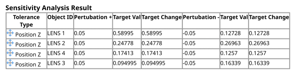
Sensitivity analysis is a method in which we test our performance metrics when each parameter is applied with the highest and lowest values that it might reach according to its tolerances when all the other parameters are set to nominal values.
For example, let’s assume we have a 4-lens system with one degree of tolerance on the optical axis as in the sketch below (simulated in Quadoa optical simulation software).
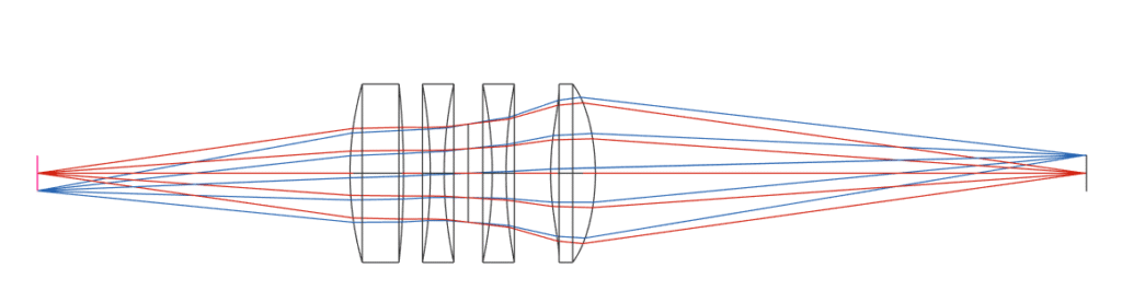
The sensitivity analysis in this case will include 4 rows with 2 entries in each, the first row the metrics results for lens #1 with its high tolerance and low tolerance applied and lenses #2 – #4 are stationary in nominal position, for number 2 with lens #2 tolerances and you may already guess what’s in rows numbers 3 and 4 ![]() .
.
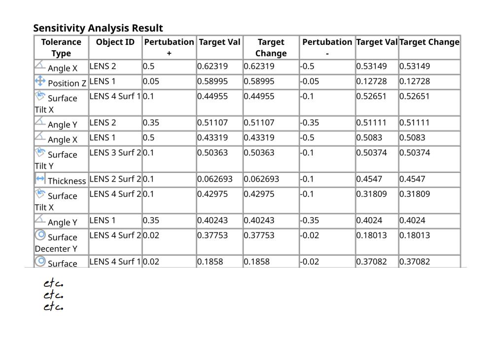
Now imagine that each lens has positioning tolerance in all 3 directions as well as rotational tolerances. That’s already 6 rows per lens, with two values in each row. Add to that manufacturing tolerances over the lens’ surfaces, the lens’ refractive index, lens’ optical axis (vs. mechanical axis) and we can easily get to 12-15 rows per lens.
This method has a very big advantage of giving us the information we need to identify where are the system’s most sensitive parts. In addition, it gives us a hint where our alignment or motorized axis should be, as we will detail later on.
What it does not give us is the overall performance of the system, since it moves only one tolerance at a time.
For that we have to use the Monte-Carlo analysis.
Monte-Carlo Tolerance Analysis
Definition from claude.ai:
A Monte-Carlo (MC) analysis is a computational method that uses repeated random sampling to model the probability of different outcomes in a process that cannot easily be predicted due to the intervention of random variables.
In human words it means that the MC analysis takes a bunch of parameters, each in its own range, and gives it a random value inside that range according to a predefined distribution.
When we apply this method to a fully blown system we get the performance metrics of the system in light of a certain state of the system’s tolerances – each parameter with its own value.
If we run enough iterations of such states, we can extract the average, min, max and STDdev of a certain metric in a system with tolerances. See blow the output for our 4-lens system with 15 iterations Monte-Carlo analysis.
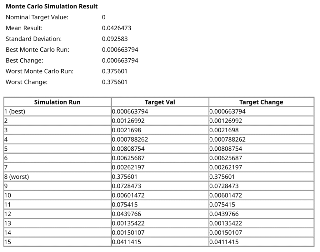
The MC analysis is a very powerful statistical tool that allows us engineers to predict, a priori, our system’s performance in design and simulation stages. It is used like in our example for engineering, manufacturing (yield assessment), in risk assessment, in finance and many other fields that require statistical evaluation of a certain state.
What the MC analysis cannot do is tell us which parameters are the main contributors for any misbehavior of our system performance.
That is why Sensitivity analysis and Monte-Carlo analysis go hand-in-hand, simply because they complement each-other.
BTW, in optical systems these two methods are considered a must for any optical design so, as such you may find them as inherent tools in all optical design SW such as Zemax Optics Studio, Quadoa, Code V etc.
Monte-Carlo and Sensitivity Analyses are as good as their inputs
Remember, both the MC and the Sensitivity analyses are as good their inputs. If we enter wrong or non-realistic tolerances into the simulations or we omit some contributors from the analyses we will get essentially meaningless results that do not reflect reality. We must have all the elements in the system that have some kind of a tolerance and the corresponding number for the state of the system we simulate.
If the materials that we use thermally change their shape or refractive index we must assess that change and insert it into the tolerances. If our manufacturer can keep the glass thickness in the range of ±5% we must enter that into the tolerances. Don’t assume anything to be negligible, at least not in the beginning. Put everything into the analysis and only after proven to be negligible remove it from the analysis so as to save time and resources.
One important note though: it is very important to exactly define the purpose of the simulation in order to have the right inputs into that simulation. Without a clear goal the simulation may turn out to be a waste of good computation power ![]() .
.
Sensitivity Analysis Timing During Development
One question that always rises during the development process is when exactly should we conduct our sensitivity analysis?
The trade-off is simple – as we go along the design process we have less unknowns for the simulation so it is more accurate however, the cost of changes in order to correctly respond to a simulation output is higher.
There is of course one step in the design, especially in complex optical systems, where we must have these analyses done and ready to our satisfaction: before manufacturing of the first prototype system or before going to production, this depends on your transfer to production model.
In addition, I personally like having these analyses done also quite early in the design process so as to make sure that the design converges into something manufacturable that complies with the system requirements.
Alignment DOF vs. Dynamic DOF vs. Static
The following section refers mainly to optical system design but you may copy the line-of-thought into other fields such as mechanics and even SW & electronics.
As we all know, quite a few optical systems require alignment during manufacturing, on site and even in periodical maintenance. In a lot of these systems there are also dynamic Degrees of Freedom (DOF) that move and compensate for inaccuracies during system operation.
To make sure we are on the same page, in all of my posts a DOF is any kind of physical property (usually mechanical, but can be electrical or any other) that may controlled, changed and set either by a human or programmatically by a feedback loop in the system.
How do we determine which DOFs we need for alignment, which DOFs are required for system operation and which elements we just position in their manufacturing tolerances?
Before we dive into these topics there is an additional concept in tolerance analysis we have to introduce – the Compensator.
A compensator is a dynamically changeable set of parameters with a dedicated metrics as its feedback which is not necessarily any metrics for the system performance. The simplest compensator we use all the time is the focus mechanism in our cellphones. The focus feedback is the sharpness of the edges in the location where we touched on our cellphone screen.
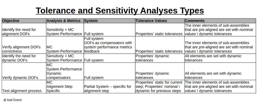
Alignment Process → Positioning
To assess initially whether we need any kind of alignment DOFs we simply do Sensitivity and MC analyses over the system as a whole with the system performance merits as targets and with the static tolerances of all the elements in the system. Note that in the case of a system of sub-assemblies, where each sub-assembly has its own pre-alignment procedure we have to consider these sub-assemblies as already positioned in nominal, hence for the understanding of alignment DOFs we will apply them with nominal values or dynamic tolerances in the sub-assembly level.
If all the metrics converge into our requirements ranges then there’s no need for any kind of DOF.
The story gets complicated when the metrics do not converge to our target in all the cases. Let’s divide it into two cases: production systems where we may accept some yield loss and systems that must perform within our requirement for every system we manufacture.
The easy case is when the expected yield loss is above our minimum required yield such that we do not require any alignment DOFs.
When the realization that DOFs are required has sunk-in, we must start identifying which set of DOFs is required in order to get the system aligned into the required performance limits. There isn’t a right and wrong way to do that – we start by looking at the Sensitivity Analysis and eliminate the main impactors i.e. add them as DOFs. Only then we address the smaller impacts. The choice of DOFs for alignment is an art but it has a direct feedback. When we’ve decided on a DOF set we then have a MC analysis with these parameters as compensators. If we get a 100% compliance it means that our DOF set is correct (maybe not the minimal set, but correct).
Each step of the alignment is a sub-system in itself
There is an important design step here that very often gets overlooked. Once we have an alignment process, we must verify that each step in the alignment process converges. In quite a few optical systems, especially the complex ones, we do not assemble all of the components and start the moving the knobs of the alignment. The assembly and alignment process is done step by step. When it comes to the relevant MC analysis, we must simulate our current step.
For example, if we build our optical system lens #1 and #2 and align lens #2; then we assemble lens #3 and align it and only then assemble lens #4 to give us the full system. In this simple case we would have to run MC on 3 sub-systems: lenses #1-#2, lenses #1-#3 and the full system.
Let’s break it down. The MC needs to have metrics and tolerances. The metrics for at least the first 2 sub-systems cannot be the system’s performance metrics, simply because the system is not fully assembled, so we will have to come up with metrics that resembles our measurement method for these particular steps – if we use an alignment jig, that jig should be a part of the sub-assembly in the MC analysis.
The tolerances of step N would be the static (positioning and manufacturing) tolerances of step N for the newly assembled elements in that step however, the tolerances values of all the previously assembled element of steps 1…N-1 would be the either nominal values or dynamic tolerances, since the previous alignment steps already set them correctly in the sub-system.
Stability → Performance and in-operation feedback
There is a very big difference between an alignment process that may take several hours of even days but rarely executed and a calibration process that constantly performs recovery for fast changes in the system. In the cases where this calibration requires a DOF we consider this DOF as a dynamic DOF. In our imaging example, focus mechanism is a dynamic DOF. Note that I ignore requirement-derived DOFs for example, if we require 2 different apertures for f# 4.5 and f# 8 we must add a DOF to the system for that regardless of any performance issues we might have.
In order to assess if we need a dynamic DOF we execute Sensitivity and MC analyses and check whether our metrics are inside the required limits. If there are deviations from the required performance we use the sensitivity analysis to identify which DOF needs to be dynamic and setup a feedback mechanism in order to fix that DOF during system operation.
We must find the DOF subset that fixes all out-of-spec items
Obviously, we then have to verify that this DOF indeed fixes our problem. This is done via MC analysis with the DOF and its metrics that act as a compensator. If there are still out-of-spec values in the performance metrics we would have to repeat the Sensitivity and MC analyses, this time with the compensators previously defined to understand which DOFs need to be added to the list of compensators.
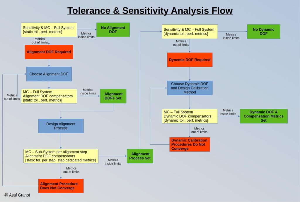
I realize it sounds a bit confusing and there are some iterative tasks in the process. If we take the tolerance analysis as a whole, the long path flow looks like the following:
This fully-blown flow is sometimes an overkill for simpler systems and a shorter flow may suffice. In these cases, a flow where we skip the alignment process MC analysis and the dynamic DOF MC analysis would be something like this:
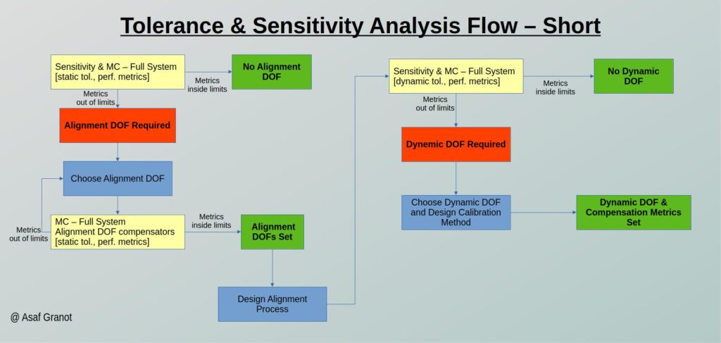
As usual, nothing in these flows is a must. These flows are suggestions that worked for me in different kinds of projects however, if another short\longer process with different inputs and outputs works for you, knock yourself out.
MC Analysis vs. General Technical Budget
One may ask how sensitivity or MC analysis differ from any other technical budget that we mentioned previously in this blog; In their essence they seem the same: both have some quantitative metrics, both end with an answer “comply / not-comply” for that metrics.
The difference between them however is that sensitivity\MC analysis is the tool while the error budget can be considered as a system requirement. Error budgets in the system level are a very common breakdown method for sub-system level requirements but I have never encountered an error budget for different stages of alignment and very rarely have I seen engineers going through building a complete error budget just to find which DOF are required for one element in one of their sub-systems.
That’s it for this post. The task of tolerance analysis is an art – to identify the properties that affect the system performance, to quantify their static and dynamic tolerance and accordingly identify which degrees of freedom are required for the system. It is not an easy task and may well be the difference between a working system and a useless assembly of metal and glass.In the process of the tolerance analysis all kinds of design obstacles are removed: non-converging alignment process, inaccurate calibration flows, wide tolerance manufacturing and so on.
I truly hope that this post will help you in your next system design and will save you a few erroneous manufacturing and assembly iterations where the system’s performance does not comply with the requirements.