
We are still exploring the importance of the alignment procedure in system design. After covering, in theory, the different ins and outs of alignment procedure and why it is so important, it is much easier to understand the theory when looking at a real-life-like example.
If you have not read the first post in this series I strongly suggest you do since this post is the practice of the theory presented in the first post. I also recommend reading this post about tolerance analysis for a quick recap because this topic is relevant to this post’s content.
An example – Microscope
First, we will take as an example a simple microscope system: an objective, a tube-lens and a camera to resolve properly 1um features i.e. 500lp/mm an objective NA=0.8 (diffraction limit is at the 0.5um for such a system so we’re on the safe side).
We would like the MTF to be greater than 0.25 in a 400um FOV (in the simulation I added 60um).
The target is omni luminescence i.e. no need to deal with the illumination at this point.
For this example, I have taken the objective from patent US04379623 and a tube-lens from patent US5699196 and adjusted, “a bit”, their shape and parameters to fit our example simulation with an AVT Manta G-419 5.5um pixel size.
This solution is not fully optimized to the best performance we could have gotten in a similar lens structure. I kept it not ideal on purpose.
So, we ended up with a X27.5 optical system, i.e. a 1um on target will spread to 27.5um. On a 5.5um pixel size we get 5 pixels for minimum resolution – 2 pixels more than the minimum required dictated by nyquist but we can live with a bit of spares for the sake of this example.
All the simulations were done using Quadoa optical CAD.
To simplify the example, I will treat each of the lens assemblies – the Objective and the tube-lens – as pre-aligned by “an external vendor”. Note that in custom-made elements this assumption cannot be made.
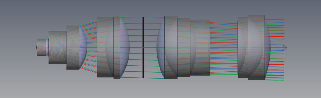
The objective standalone and the assembled system look like this:

Tolerance Analysis
Simulation Mechanical Pivots
Before showing the results of the tolerance analysis there is a little update I had to do to the model – defining the mechanical pivot points of the different elements to something realistic.
A mechanical pivot point of an optical elements usually represents the mechanical mount of the element in the optical system.
It means that if we get that the rotational tolerance of our tube-lens is an exaggerated 10 degrees, we should also verify what is the point around which these 10 degrees rotate.
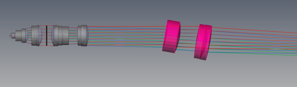
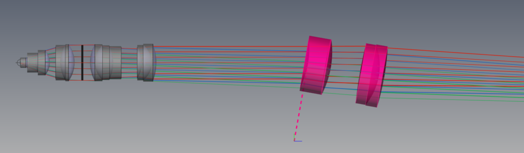
In our example a mount that is positioned 20mm below the tube-lens’ first surface represents a reasonable non-rigid mechanical mount (-20mm in the y direction) and an even more reasonable rigid mount would be 20mm below the assembly and 20mm inward (-20mm in the y direction and 20mm in the z direction).
See below how the same 10 degrees rotation is different for 3 different pivot points that represents different mechanical mounts. The Quadoa SW even shows the location of the pivot when dealing with off-axis elements in a purple dashed line:
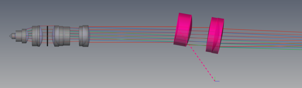
Note that there are cases where the tolerance movements of the elements are not the same as the mechanical DOF that was created to fix them. In our case, for simplicity of course, we will treat them as the same.
BTW, you should expect competent mechanical engineers to design the DOFs such that the movement pivot of each DOF is around the center of the optical element and such that all DOFs are orthogonal to one-another. This pivot task is not always possible because of many constraints that may exist in the system, but do not compromise on the orthogonality – without it the alignment task becomes a continuous nightmare.
Tolerance Analysis Results Turn into Alignment Procedure
I have taken the system’s performance as our target resolution MTF. I would have shown the results here but quite a lot of the Monte-Carlo iteration ended up with effectively zero MTF results because of ray cutoff in the system.
So, alignment is required!
After following very carefully the process we described in this post the conclusion was that the following DOFs need adjustment if we pivot our target i.e. if not DOFs are applied to the target and we take it as constant:
Objective tip, tilt, x, y, z; Tube-lens tip, tilt, x, y, z; camera plane tip, tilt, x, y
There is a catch here. We could address the optics as a whole and set the optics’ pivot as the camera plane. Then we will get a different list:
Objective tip, tilt, x, y; Tube-lens tip, tilt, x, y, z; Optics tip, tilt, x, y, z
But if we have already moved the whole optic vs. the target and the target is only a very small 400um, it would be wiser to have the translation x, y, z DOFs move the target and not the whole optics so we get:
Objective tip, tilt, x, y; Tube-lens tip, tilt, x, y, z; Optics tip, tilt; Target x, y, z
The trick here was to address the geometry of the different DOFs and understanding that camera movements are equivalent to whole optics movement which in turn equivalent to target movements. Note that the need for z DOF switched from the objective to the optics and then to the target, since the objective is planned as infinity corrected objective.
Why is all that so important?
When addressing the alignment procedure, we have to be open-minded to lock DOFs on the one hand and unlock them on the other hand, according to our needs. In our particular example we have an inherent feedback sensor – the camera. We may as well use it as our pivot and align everything to it.
The other option is to have another sensor as feedback for our alignment as a jig and then remove it. It is indeed a viable option but, in our case, not optimal.
Alignment Procedure
After we’ve set the optics’ pivot, we have more than one approach to design this procedure.
The first and very straight forward method is to assemble all the parts, put a calibration target in front of the objective and start tweaking the DOFs until reaching the require performance.
Don’t get me wrong, with “only” 3 optical elements that method could work. However, this is an iterative and frustrating process with many DOFs that have the exact same result in our feedback system (the camera image). For example, how would we differentiate between the tube-lens tip and the camera plan’s tip?
In other words, alignment processes that start with a prayer are not considered good practice.
The second method in our case would be the following:
- Fix the camera
- Align the tube-lens to the camera
- Align the objective to the tube-lens and camera
- Fix the tip/tilt of the objective to the target plane when the target’s x, y, z are dynamic to fit a set of targets
I do not want to go into each and every little detail in this procedure because it will take forever. I will concentrate on two specific points.
In step #2, to align the tube-lens towards the camera we would need a collimated illumination source and by analyzing the image of the source in the camera we know how well our alignment is. See the simulated image.

However, in practice we do not get this beautiful bundle of rays. If we use a 3mm diameter laser the ideal image would look like this:

A realistic random placing of the illumination would have an angle towards the optical axis of the tube-lens and would look like this:

In other words, when introducing this collimated light source, we have to take care of its position against the real optical axis of the tube-lens assembly otherwise this process would not converge into our desired performance.
There are ways to do that of course (the first method that pops into mind is centering the beam on the front surface via reflection of the laser off that surface – like how an autocollimator operates) but that’s not the main point of the discussion. The point is to cover this in the alignment procedure otherwise the procedure is not bound to converge.
An alignment procedure that does not converge means system failure.
Extension of the Microscope example
The is an extension of this simple microscope example that I would like to make for the purpose of emphasizing the alignment steps closure point.
Let’s introduce a through illumination path to our design with a collimated light source and a beam-splitter, as follows:

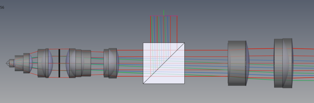
We will not go into the process of the DOF choice all over again, but there is an important warning here: even when inserting an allegedly parallel surfaces element in the “infinity zone” of this system it does not come without a toll. The tip/tilt angles may cause beam displacements; the illumination beam has to be precisely aligned with the collection FOV and so on. In a non-ideal system this beam-splitter insertion might severely impact the imaging performance of the system.
In such a case the “easy” alignment solution would be to align everything as before, then insert the beam-splitter and align the beam-splitter DOFs until the same imaging performance is achieved as before the beam-splitter was inserted and only then apply the illumination and calibration its angle and location.
However, what if the alignment had already been performed for the tube-lens had compensated for a non-ideal “infinity zone”? What then? It may result in an optical path that cannot be completely aligned into specs with only the beam-splitter DOFs and require re-adjustment of the tube-lens’ DOFs or the objective’s DOFs.
A quick check in the simulation showed me that it is indeed the case in our example, especially when applying also manufacturing tolerances to the cube of the beam-splitter, which means that we need to re-design the whole alignment process.
That would also mean that if we added this illumination extension in an existing system in field we could end up with a non-operating system in the field, only because we have overlooked a potential non-closure in the alignment process during design.
An addition of elements to an existing alignment procedure does not guarantee that previously aligned elements stay as much.
That’s it for this post.
In this 2-part post-series we’ve explored the need for proper and accurate alignment methods and processes for our systems, up to the point where a not-suitable process might make a system non-operational and might even kill a project.
An optical design without an accompanying optical alignment procedure is only half a design!