Over the years I have been involved in many projects that included vision modules in which each vision system resolution was defined differently. In most of these projects the bottom line in the development processes was that either the optical designer had to translate the resolution requirements to optical language or that the end results of the optical design was an overkill in terms of performance (and probably costs wise as well) to whatever the system really needed. This post is designed to clarify how optical resolution should be defined, what the different parameters to take note of are, and mainly how to communicate with us (the optics experts) in the same vision systems language. It is funny sometimes to witness such conversations when both sides strongly argue their case although they refer to the exact same technical issue in two different languages or methods, when they only needed to talk about resolution via MTF.
Note that there is more than one way to define the resolution of an optical system in “optical technical language”, obviously not all will be covered in this post.
When we create a set of technical requirements for a vision system, if we did our characterization for initial system requirements properly, we usually end up with the smallest element to be resolved. So great, we know we would like to have a 4um lateral (XY) resolution, but that is not nearly enough for an optical resolution definition. BTW, we deal with optics in these posts where the Z axis is referred to the optical axis or focus axis unless stated otherwise.
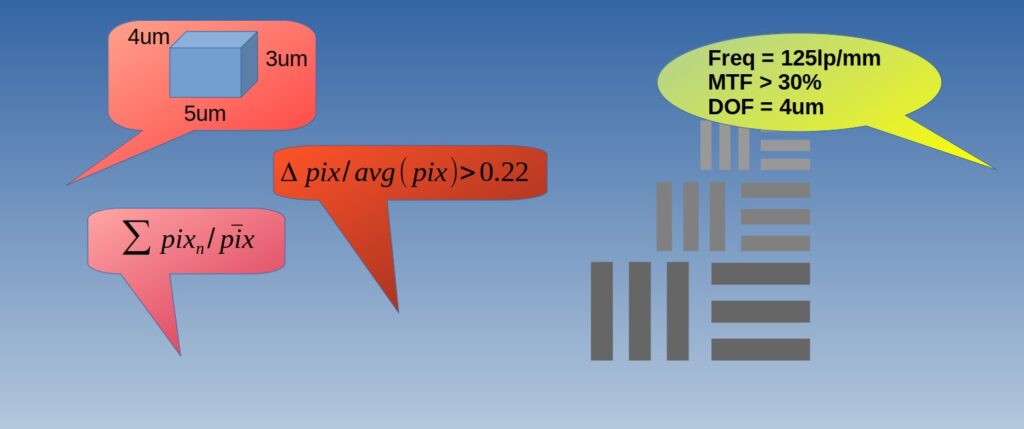
Every vision system resolution definition must not only have the smallest element to be resolved but also the Depth of Field (DOF) for that smallest element and the minimum contrast of that element vs. its surrounding in the image. DOF will be the physical range on the focus axis where the smallest element is still resolvable in the required contrast or higher contrast. Also for that matter, it is important to define contrast between features. An industry standard is ![]() , where min and max are in intensity units. Unless stated otherwise, in your requirements, it will be assumed that that’s the contrast definition you meant.
, where min and max are in intensity units. Unless stated otherwise, in your requirements, it will be assumed that that’s the contrast definition you meant.
So, in our case we would say that our optical system requirement is 4um smallest element, with a DOF of 5um, in contrast of 30%.
Tangential and Sagittal Planes
I will keep this caveat brief as to not deviate too much from the main subject. The tangential plane is the plane that contains the optical axis of the system in an off-axis point on the object. The sagittal plane is the plane perpendicular to the tangential plane. See the sketch below.
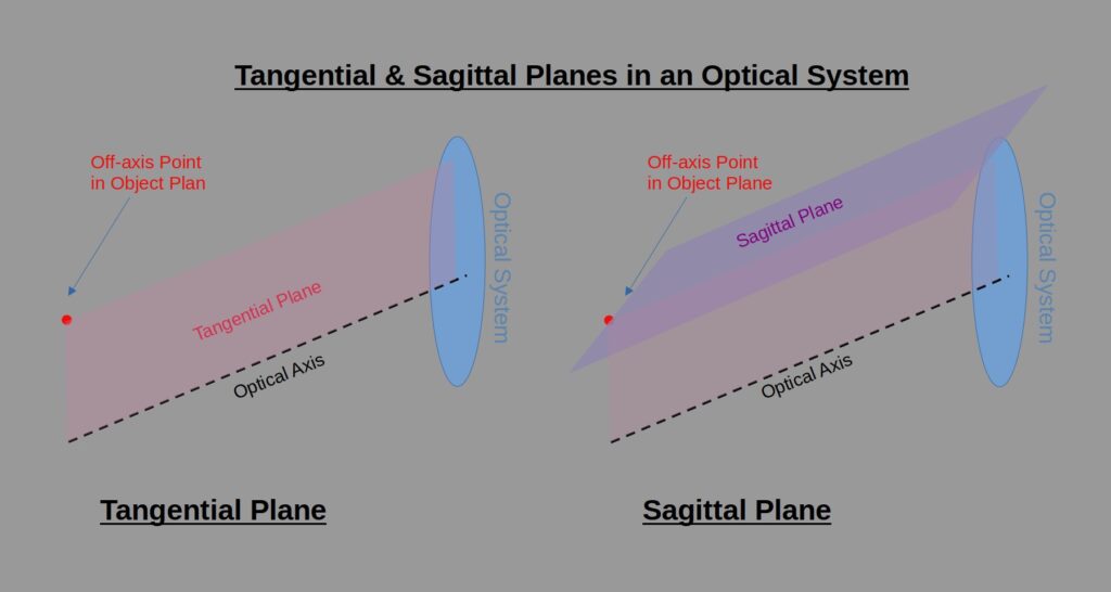
With respect to this post’s contents, it is sufficient to understand that there is a difference between the optical performance of each plane, as manifest in the different graphs below. I will cover the different aspects of these two planes in another post that will discuss optical aberrations.
MTF as a Measurable Parameter for a Vision System’s Resolution
We should always keep in mind, regardless in which discipline, to have our technical requirements measurable. A good technical requirement is one that we can measure and verify whether the system complies with this requirement or not and to measure it we must have some kind of a scale.
When it comes to the resolution of an optical system, Modulation Transfer Function or MTF is that scale. You may also encounter the term Optical Transfer Function or OTF, which is essentially the same as MTF for most vision purposes and the only difference being without the phase element.
The OTF \ MTF represent how different spatial frequencies pass through our optical system and how, eventually, they are manifested in our image. Refer to Wikipedia for a more comprehensive explanation. The bottom line is that via the OTF / MTF we can simulate and measure an optics’ spatial resolution. See below of how to measure the MTF.
We can also find references to the Point Spread Function (PSF) which is a different method to describe the light behavior in an optical system. I will cover the PSF as a whole in another post.
Microscope Objective Example
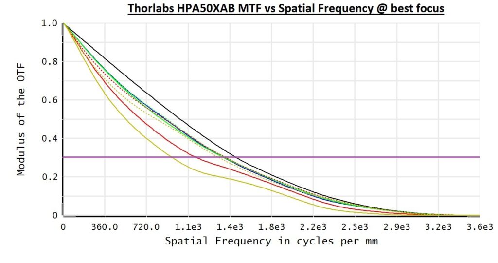
Let’s take for example, this long working distance objective by Thorlabs. All simulations were done using Ansys OpticStudio, using fft MTF calculation.
An MTF graph gives us the MTF value i.e., contrast vs. spatial frequency in line pair per mm (lp/mm). If we look at the MTF graph at best focus we get that the 30% contrast in the most demanding field (240um-tangential) is achieved at 940lp/mm, an equivalent of around 0.53um line width and lower. The purple horizontal line represents the 30% contrast lower limit in all the graphs.
The above graph does not tell the whole story. It is practically impossible to get our object plane as a whole to be all inside the best focus plane with no tolerances. That is why we define the DOF. We can systematically guarantee that our target object will be all inside the DOF range. So, let’s look at the through focus MTF graph which gives us the MTF per a certain spatial frequency vs. different location on the optical axis i.e., focus points. The following graph shows the through focus MTF for 125lp/mm which is an equivalent for our required 4um line width.
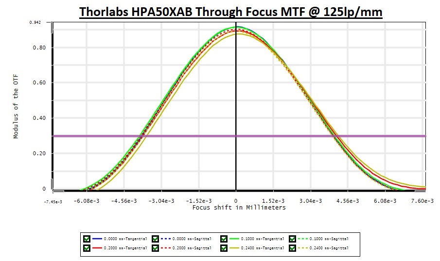
We can see here that in the same most demanding field our DOF will be ~7.2um for an MTF of 30% or higher which is definitely sufficient for our purposes as we prescribed above. The important note here is that it is not even near the 940lp/mm we got when we looked solely at the best focus MTF graph. Had we have given the optical designer only an absolute resolution target without the DOF we would not get the required optical performance.
We could also look at the same objective lens from another angle and check what the maximum resolution we would get if we needed to operate this objective lens in a DOF of 11um.
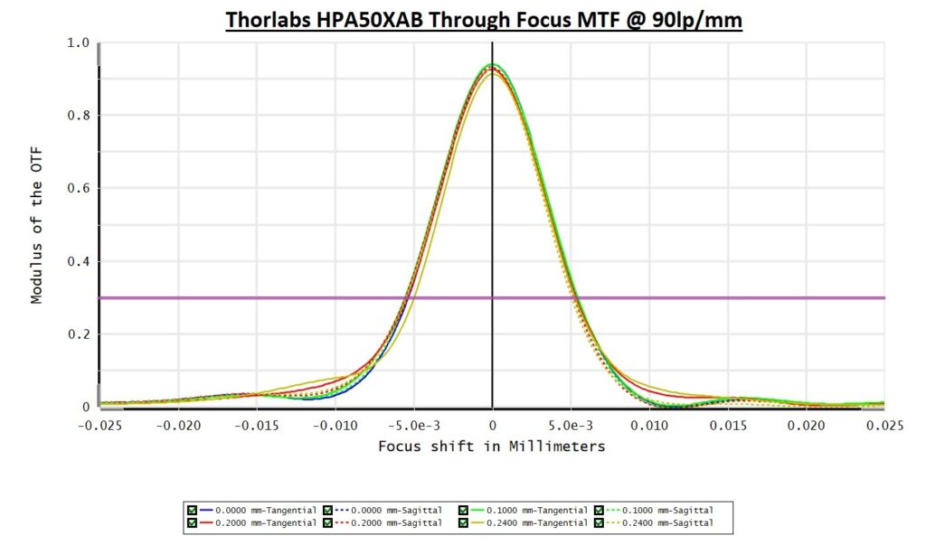
The graph above, depicting the through focus MTF for 90lp/mm, answers our question. Just to give you a taste of the work done behind the scenes and that is done on an off-the-shelf objective, of course, I had to iterate using different frequencies until I got to this answer. The effort involved in reaching this in a custom lens that has its own design is huge especially in complex multi-element optical designs such as microscopy and telescopy.
How to Measure the MTF
In essence, the measurement method of the actual MTF of an optical system is quite simple. We take a test target of our choice, insert it correctly into our optical system, and measure the contrast between light and no light conditions of the particular target. The vertical lines image would look something like this in a USAF 1951 target:
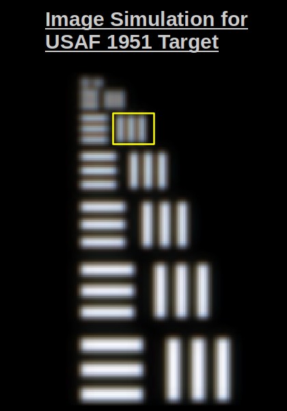
If we look at the gray level profile of the 3rd from the top vertical bar target (marked in yellow) it looks like this:
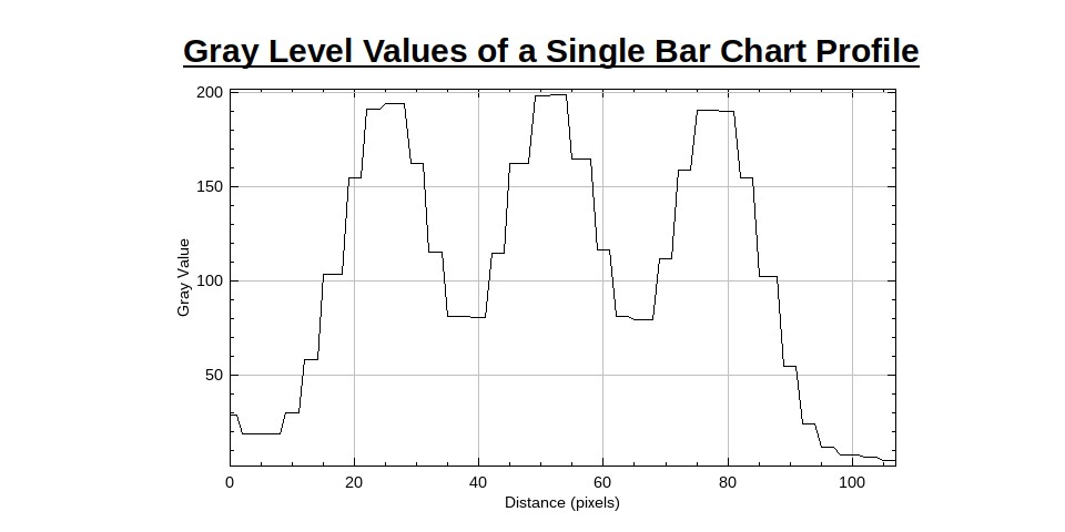
So, we can clearly calculate that for this particular target the contrast is 114/274 = 41.6%
In many cases you would like to subtract the dark signal from the calculation of the contrast such that the calculation would look like ![]() . It is not a must, but it is anyhow a good practice if you subtract the background noise or dark noise from your image in your image processing.
. It is not a must, but it is anyhow a good practice if you subtract the background noise or dark noise from your image in your image processing.
In order to exactly test our definitions as we simulated in our example we would choose an USAF 1951 High Resolution target like this one, but there are many other target kinds to choose from here for example. As our example also includes DOF definitions we would have to put either the target or the objective on an accurate stage in the Z axis and take images of the target in different focus locations and in different field locations on the optical axis.
It is also imperative to include in the measurement system the parameters that are important for your optical system – if the algorithm you are using is sensitive to defocus image, measure the defocus image and quantify it (I personally encountered this sensitivity in more than one optical system). If there are different performance factors for different fields of the image, make sure to cover those in your measurements as well.
Important note: it is crucial to make sure that the alignment of the target, moving parts and the optical system is perfect when measuring an optical system performance. In the most critical aspect of the system, it needs only one element’s location or alignment to be off to take our measurement on a path that will lead to incorrect conclusions. In the difficult cases, even if it is not trivial, make the effort.
I hope I have managed to convey one important aspect of resolution in vision systems and how crucial it is to cover all of your requirements with the optical experts in the same technical language. It may be an effort in the beginning of the project design but the effort pays off.