
Our target is moving! We have already established in previous posts that the task of matching a camera to an application is a challenge. To follow up on this statement, in this post series we will explore the camera shutter technology – global shutter vs. rolling shutter vs. event-based (which does not involve a shutter whatsoever but still participates in this competition), where the two different shutters are coupled with the camera exposure. In this post we will focus on global shutter and exposure effects on a moving target.
We will use an unorthodox moving target for the purpose of the posts in this series – a 4 blade mini-fan custom-made for this experiment. I could have used the banal moving car example but my Lamborghini was not available this week ![]() .
.
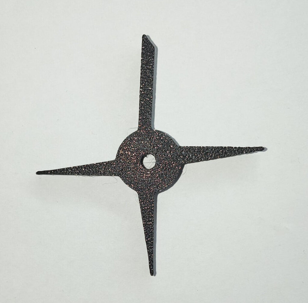
You may notice that in this particular fan one blade has a different shape to the other 3. That is so as to be able to identify that particular blade when using a narrow field-of-view (FOV). We will not use images of that particular blade; it is there only for the ease of the measurement flow.
For all the images taken in this post I used a X5 Mitutoyo objective. The camera used in this post’s images acquisition was the IDS UI-3250CP Rev. 2 camera provided by courtesy of OpteamX. The illumination used was cold white light LED wide angle light source.
The Global Shutter
Global shutter refers to acquisition simultaneously of all the camera sensor pixels, and where all the pixels in the image will experience the same absolute and relative timeline. That means that when we set an exposure of 50ms to a certain a global shutter sensor all the photon collection for all the pixels will start and end at exactly the same time.
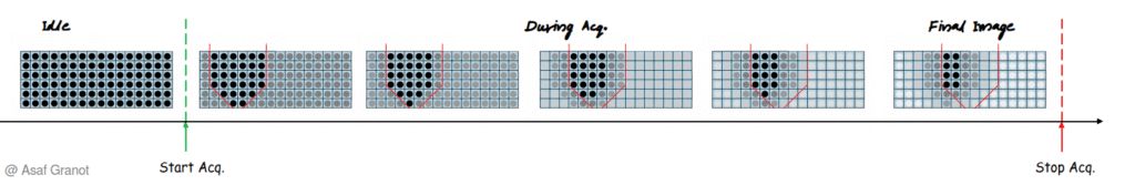
See below the image build-up evolution in time for a global shutter sensor. Note that I sketched the image build-up over time and not the pixel readout so the sketches here are different than those customarily used in the industry but I somehow think this is a better way to convey the subtle differences between the technologies.
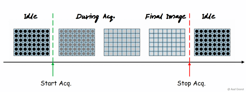
So, in practice, if we illuminate the sensor with a spatially uniform light, we will get a uniform image even if the illumination intensity levels have deviations in time. All the pixels in the sensor are exposed to light at the exact same time.
Note that there are sensor implementations where the sensor readout is done sequentially even if the shutter is global, where the pixels are still gathering photons which adds a rolling bias to the intensity of each pixel. We will not discuss nor show examples of these implementations in this post since they are not mainstream.
For the purpose of this post this relatively short explanation will suffice. When introducing the rolling shutter, we will go into more detail of the global shutter operation at the sensor level.
Static Target & Illumination
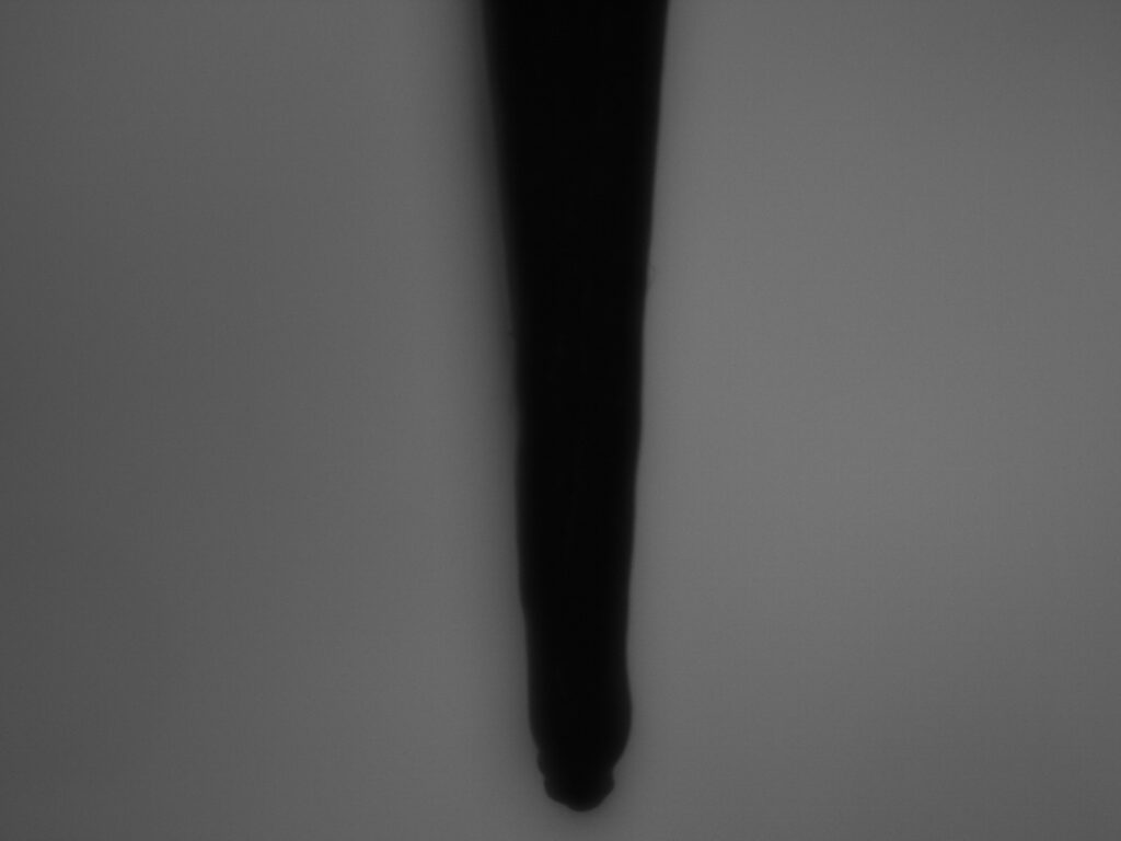
Just for reference the static image of the relevant blade looks as follows:
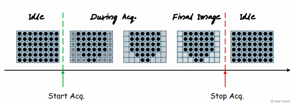
So, if we take the build-up evolution as before with the existence of the tip of the blade we will get the following flow:
Moving Target
When dealing with a moving target with a global shutter camera the quality of the image is simply a matter of optimizing the exposure time to the object speed over the sensor plane.
When we want to “freeze the moment”, that is get a static image of the moving target, we would have to make sure that our total exposure time per image is under the time it takes our target to move a significant distance in the image before it gets blurry. Blurry, of course, is a matter of definition, so I will use some images with different blurring levels for you readers to decide which is which.
In the following images the fan was rotating and the different images were taken in different exposure times:
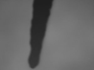
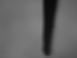
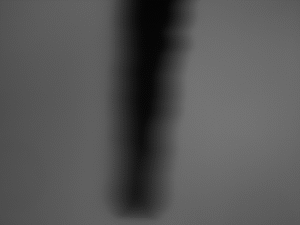

We can clearly see that with the exposure time of 0.1ms the image is very close to static, i.e. the movement of the fan blade was less than the resolution available for us in this imaging system. When we go up to 0.25ms exposure time the edges of the blade are not as sharp as in the image taken in exposure 0.1ms but we can still accurately locate where the blade is. At 0.5ms exposure time things get blurry by any definition of the word – we cannot tell where the edges of the blade start and where they end, however we can still clearly identify where the center of mass of the blade is in the image. When we go up to 1.5ms exposure time the objects are already so blurry that we cannot really identify what is passing through the camera’s field-of-view.
To better explain this phenomenon, take a look at the following set of sketches. To assist in understanding the movement of the tip, the edges of the tip are marked in red in each image. The different shades of gray represent the gray-level of the pixels very much like a real sensor gray level.
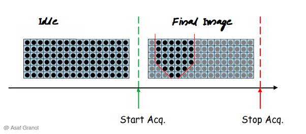
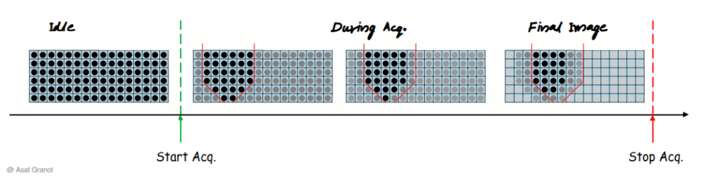
The first sketch shows a very short exposure where the resulting image is in fact the static tip of the fan’s blade.
In the second sketch we took a longer exposure time where the tip travelled an equivalent of 3 pixels during the exposure period. In this case we see that the edges of the tip are already greyed out but the center of mass of the tip enjoys black pixels since these pixels were not exposed to any light.
In the third sketch we can see that the edges are completely greyed out and even the center bulk of the tip shade is very narrow in comparison (2 pixels wide vs. 6 pixels wide).
Avoiding Blurring with Global Shutter
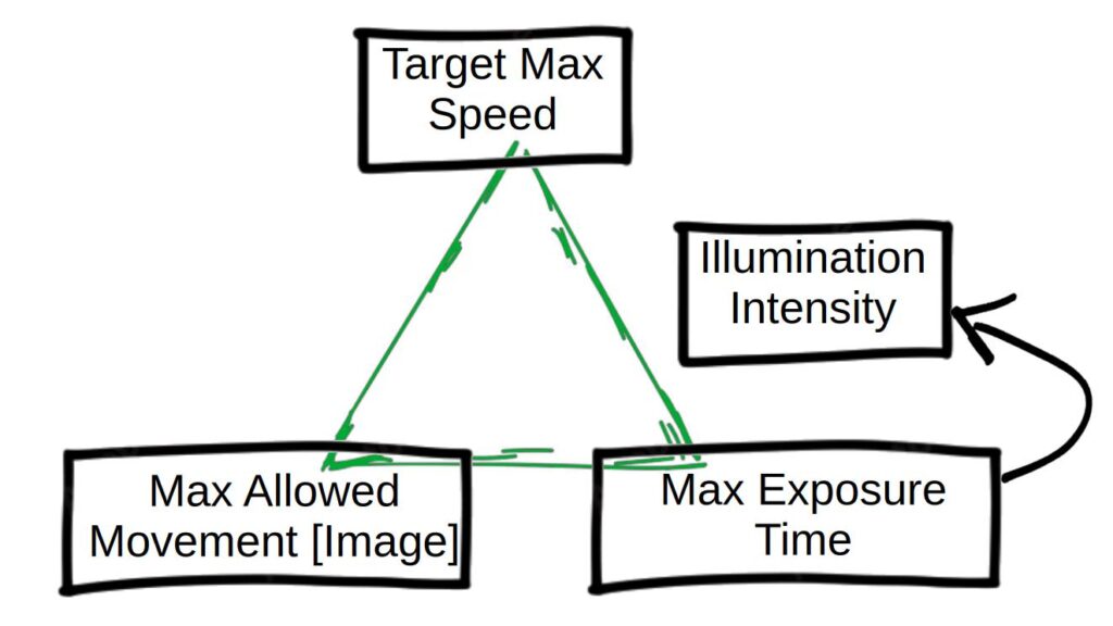
From the optical engineering point of view the solution for motion originated blur is quite straight forward – correctly calculate your maximum allowed exposure time! There is a triangle of dependency between the target maximum speed, the maximum allowed movement of the target on the image plane (in pixels) and the maximum allowed exposure time of the sensor.
Note that shorter exposure times may impact your required illumination intensity in order to have a viable signal to begin with. Although I did not mention it previously the illumination is a part of the game (for example, in the very short exposure times I had to use significant gain in order to achieve some kind of an image with reasonable contrast).
Side Note – FPS
Although not directly related to this post’s line of thought we cannot talk about exposure without mentioning the frequency of the sensor acquisition – frames-per-second (FPS).
The FPS will obviously be bound by the maximum exposure time (1 / exposure = max FPS).
Having said that, on the one hand the fact that we have a 1ms exposure time requirement does not mean that our application requires 1000 FPS and on the other hand, having an optimal “freeze” exposure of 10ms for movement and lighting does not necessarily mean that a 100 FPS will catch the scene to our utmost satisfaction.
A very nice example of the latter can be found here:
Remember that FPS gives us the resolution for changes in the time domain along with the exposure. This resolution is part of the application requirement. To measure correctly Usain Bolt’s 9.58 seconds world record we cannot use a 100FPS camera even if a 10ms exposure time is enough to take a beautiful non-blurred image of all 8 athletes on the runway.
That’s it for this post. In the next post we will explore another sensor technology and compare it with the global shutter technology we explored in this post.