Once in a while we are exposed to a new technology that changes our perception and our approach to a certain field. In my opinion such is the event-based camera technology. You may also find the term neuromorphic cameras or sensors used instead but they are the same. In a nutshell, it is having the flow of bytes of the camera make use of only a selected handful of pixels each packet instead of the entire sensor or the Region of Interest (ROI) of the sensor and specifically in neuromorphic sensors – only those that experienced some kind of a change – an event.
Although the concept of event-based sensing has been around for about 10 years this technology is not as yet widespread and accordingly you may find only a handful of manufacturers that deal with this sensor technology among who are Prophesee, inivation, Insightness and CelePixel, each with its own unique tech. We can only see now camera manufacturers starting to integrate this tech into their products (Sept-2024).
General note: in this post series I will refer to the data analysis of all camera types as “image processing” even though in event-based cameras it is not an image per se.
What Is An Event-Based Camera?
An event-based camera is a camera that indicates a change of grey level (GL) per pixel. Each such change is referred to as “event”. The camera will then stream out on its data channel a stream of events. Each event’s packet size will be a few bytes to hold the required information: x location (row), y location (column), timestamp and the nature of the change and any other information the vendor has decided to share with us.
Unlike a classical camera that streams out an image in a known frequency (frames per second – FPS) thus occupying a known bandwidth, the event-based camera’s bandwidth will change according to the flow of events – if say only one pixel changed during the last second if will occupy a bandwidth of a packet size per second. As the number of changed pixels per second grows in our scene the bandwidth will grow but obviously up to a certain limitation which is dictated by the electronics of the camera and sensor.
Confused? Lets look at a simple artificial example:
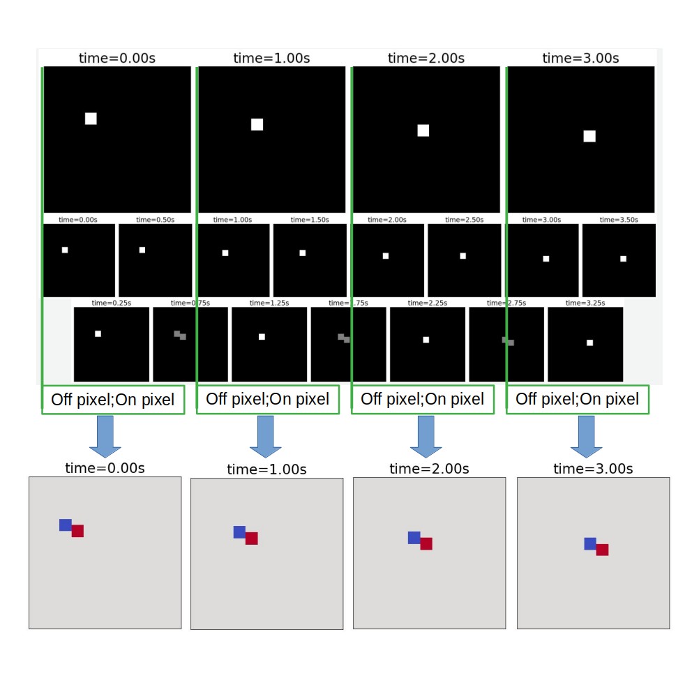
In this example we first see a quick movie of a scene. A single point is being illuminated each time in a different XY location in the scene. The first row is the scene that changes every 1s. The row presents a period of 4 seconds.
In the second row we see the output of a standard camera with a high FPS, X2 faster than the illumination point location change. To support this scene, we had to take 8 images over the entire 4 seconds of the event, 0.5s exposure time per frame. The point size is 2×2 pixels.
The third row shows the output of the same standard camera but with the synchronization of the camera image taking is shifted a bit from that of the illumination location change.
In such a case where the scene is not synced with the camera image taking, we would require a higher FPS in order to correctly get the scene images. It was not frequent enough in our case example so only half the images pictured the transition.
In the fourth row we see a flow of events. Each timestamp shows the “on” event of a certain pixel and the “off” event of another pixel. Because the points take 2×2 pixels, it will be 4 events for “on” and 4 events for “off”. The row below it is the translation into an image of the accumulated events in that particular time frame – red is on, blue is off and grey is for no events.
To sum up in the standard camera we ended up with a set of 8 images of 25×25 pixels of 8bit, i.e. 5kB / 4s, which were not necessarily synchronized and, in the event-based camera we ended up with a list of 32 events each in the order of 50bit, i.e. 200B / 4s, describing the exact same movement of the illumination. And, to be frank, we could skip the “off” events in this particular case. So, if we wanted to, we could reduce the number of events by half,.
In this simple example we may see that we have three advantages in the event-based camera over the standard camera. First, we used significantly less bits and bytes to describe the exact same scene; second, we get an inherent synchronization of the scene events using this technology and third, we do not have to worry (up to a certain limit of course), about our frame frequency.
So, What Exactly Is An Event?
As previously mentioned, an event is any change in the pixel’s GL, which means that even 1GL change will be caught as an event. However, the pixels have an inherent noise such as Shot noise and thermal Johnson noise and that on top of the scene noise so we must have some kind of a thresholding mechanism in order to eliminate these noise sources from creating a non-existent or unwanted flow of events. The exact thresholding would depend on the camera model and the scene.
Specifically in the IDS Imaging EventBasedSensor Eval-Kit ES (yes, an evaluation kit, that’s the only thing available) with the Sony IMX636 and the Prophesee metavision SDK that I will be using in this post series there are different thresholds (called biases) available for our use such as: factor for intensity change for the “on” event, factor for intensity change for the “off” event, high-pass and low-pass filters, dead time to “sleep” after an event was registered (so as not to get the same event over and over).
The camera was provided by courtesy of OpteamX.
Image Construction of Event-Based Info
The most interesting issue here is what can and should be done with these events. Suddenly, something as trivial as image construction becomes a challenge. I will explore the most common methods; each serves a different purpose. The images and movies were taken with the evaluation kit camera mentioned above and the OPT-C1618-5M lens and simple generic LED illumination.
Construct a Frame by Accumulation of Events
As simple as it sounds – we accumulate all the events that happened in a certain time window and present it. See example below of a movie of a moving laser beam from one side of the Field Of View (FOV) to the other. Each frame in this movie is the accumulation of all the “on” events that occurred in the time window of 500us. The total movie duration is 40ms. You may ignore the timestamp title – only the relevant 40ms out of a 9s movie.
It is as if we were grabbing an image in a standard exposure camera and a very fast one.
We would use this image construction method when we are interested in the scene but we do not need the information about the timing of the scene for example, movement detection.
Time Coloring of an Accumulated Frame
This is the less intuitive method of image construction. In this image construction we give a different color indication for each timestamp and accumulate all the events in a single image or movie.
The exact same movement above where we build up the image in different colors will look like this:
Or in a non-animated single image:
In both the movie and the image above each color represents a different time in the capture time-frame where the scale in micro-seconds (yes, micro-seconds!) is on the right colorbar.
The same data may be presented in 3D where the additional axis will be the time however, in this particular example of the laser spot movement the resulting movie does injustice to this presentation method. I will leave the 3D movies to later posts.
Different Coloring for “on” and “off” Events
Another way of representation is using different colors for “on” and “off” events for a time-frame very much like the first image construction method. It has the advantage of observing transient event vs. constant changes in the relevant applications. See our laser spot below, (all events are transients in our case), where in red we see the “on” events and in blue the “off” events.
Histogram Per Pixel
This is a very unorthodox imaging method which may give us information only in applications where we search for light indications from specific locations in the scene for example, if we wanted to map the pixels that experienced the most light during a specific time period in a scene. The histogram simply counts the number of events per pixel accumulated by time. When we take our moving laser spot we will get the following movie:
You have probably noticed that in all the examples of representation methods I have shown a movie representation rather than a single image. I felt that in most cases a single image does not tell us the whole story in that specific example. In the following posts in this series, where I will dig deeper into certain aspects of the image processing involved in event-based cameras, I will try where possible to convey the message via a single image.
To sum up, when it comes to representation methods, it’s really the tip of the ice-burg. I have detailed the main representation methods however, there are many more data representation methods for event-based streams that are less “image” like and more application specific. For more about representation methods, you may look here.
What is Neuromorphic Imaging Good For?
Is that the end of the “standard” camera era? Definitely not! Like every tool in our toolbox, there are the tasks that it will fit and there are those it will not.
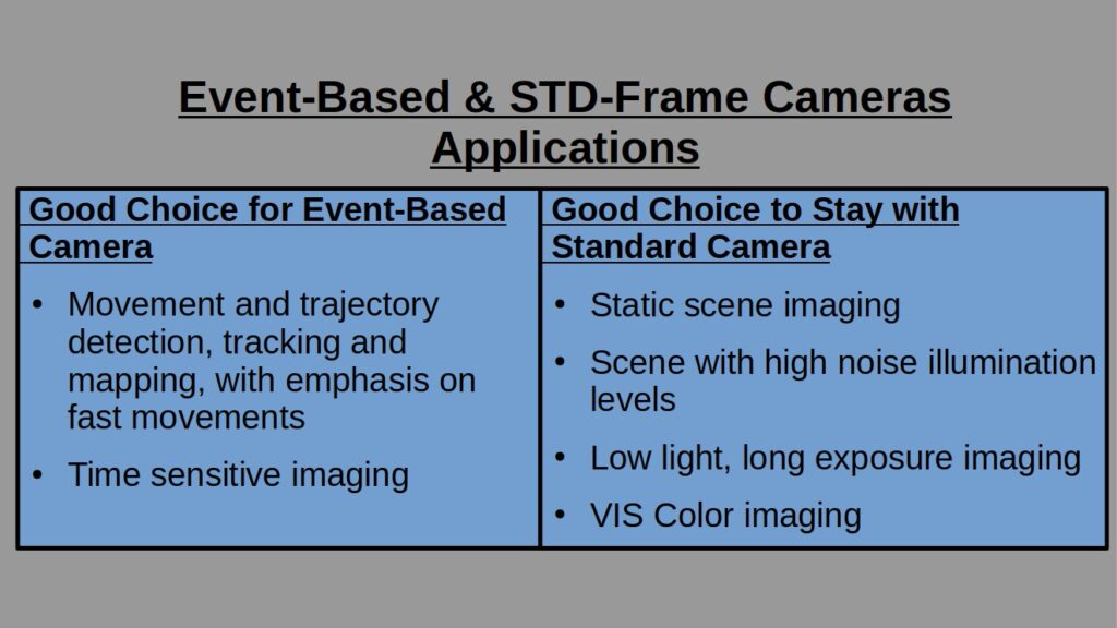
Note that you may of course use event-based cameras for each of the right list’s application but it would force you to be very creative in your image processing and would not be the best use of these camera’s technology.
That’s it for this intro, here we laid down the basics of the neuromorphic cameras. This is only a mind-opener to a technology that has many more ins and outs. In the next post in this series, we will discuss how the most trivial task in an optical setup – focusing – becomes a very challenging task.