Our starting point for this post is the very beginning of system design. A list of system requirements for our planned product already exists and now we have to develop it or in simple words to make it work.
We are past the first round with the different technical teams and/or even further along the system design. We already have a good plan as to what our system is going to look like so now, we have to guarantee to ourselves that the design is going to do what we wanted it to do to begin with. One way of course is to skip the guarantee and just assemble everything together as planned and verify that everything works to our satisfaction. Don’t get me wrong, this method works but, in my experience, it only works in very low complexity systems or jigs. But if we are looking at systems with a low to medium complexity or a higher complexity or a system of systems this method just does not work. The inter-relationship between the different components and subsystems and their correlations prevent the par-touch method from being a viable alternative.
So, what do we do? We calculate!
There are many ways to calculate technical budgets. I will cover the main 3 budget types in this post because, again in my experience, all the technical budgets are either directly one of these three or a very close variation of one of them. Remember that a technical budget is only a tool and a means to an end. Not all hammers are alike exactly as not all nails are alike. We should always pick the right tool and the right process for our project as opposed to the method of using an engineering process because our predecessors may have used it. More about that in a different post.
Technical Budget Types
Worst case – sum of extreme values
We take the worst case scenario for each contributor in our budget. We write extreme and not necessarily “max” because sometimes the worst offender is not the maximum value.
where X is the list of contributors and ext(x) is the extreme value for a single contributor.
This is definitely the safest budget calculation. If our worst case budget is kept inside our specifications and requirements this budget is definitely in the clear and we can keep that design. However, designing a system for each and every budget according to the worst case scenario may be very expensive in both engineering effort wise and final BOM wise. We must choose carefully where to follow the worst case budget.
Average case – sum of averages
As the name implies, we calculate what the average case for each contributor in our budget and sum up all the values to get the total of averages budget.
where X is the list of contributors and
is the average value for a single contributor.
Note that when dealing with the average case we should always calculate the magnitude and occurrence probability of the worst case. If the occurrence rate is acceptable systematically, we may ignore the worst case budget and take the average one as our baseline. The acceptable rate is totally application dependent. For example, if we plan a cardio mapping camera that goes directly into a patient’s heart and our device diameter budget goes 1mm larger in the worst case, a 1:1000 probability is probably not acceptable and, in this case, we must address only the worst case budget. Take the same probability for a desktop microscope in a laboratory and a 1:1000 odds would most likely be acceptable and we would keep running on the average case for that budget.
Root of sum of squares of deviation \ error
In this method we calculate the deviation of the value we measure in practice vs. the desired value (referred to as “error”) for each contributor. The final value is the root of the sum of squares of these errors. This method is the most commonly used when calculating the total noise level of a certain budget for uncorrelated noise sources. It gives us a very good indication of how well we are going to keep our system within a given tolerance. We could take the average error or the max error calculated per contributor but this depends on the probability and the severity we would like to cover in that particular budget.
where X is the list of contributors and x is the value measured \ calculated for a contributor and
is the expected value for a contributor.
The following table roughly shows where each method could be the right fit.
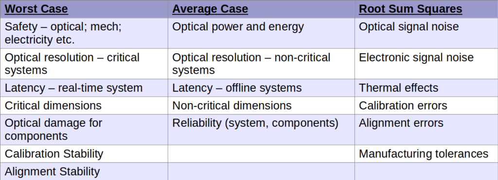
The definition of critical in the table varies from system to system. In a medical device more or less everything may be considered critical since the patient’s life would depend on it as opposed to a household device that makes coffee criticality of budgets are limited to user safety and the rest are only convenience related features.
Value Calculation Methods and Technical Budget Confidence
Not every effect that might impact our system can be measured, especially not in early stages of the project, immediately after initial requirements formulation. In many cases the impact of the effect over the budget is indirect and an additional derivative must be done. For example, we know our system’s environment temperature may rise during system operation at 15oC which causes the Aluminum optical holders to expand while we would like to assess the impact on the optical power. Multiple calculations and measurements are due here: (a) temperature rise in [oC]. (b) the expansion coefficient of the Aluminum [mm/oC]. (c) the dimensions of the Aluminum holder [mm]. (d) the movement in [mm] effect of the optical element [Watt], so that we finally get the transition [oC/Watt].
The following list, in descending order of confidence, details the different evaluation methods for a value in a budget.
- Measurement – direct or indirect measurement of the relevant effect or element in our budget. By far the best and most reliable option. We have to be careful though. When we measure anything, we must make sure to measure the exact parameter we wanted to – conduct a proper Design Of Experiment (DOE) and isolate the required parameter. It is better to admit that we cannot measure an effect and guesstimate it in the budget (see below) than use an incorrectly taken measurement which will be, as a result, used in an incorrectly assumed high confidence during the process and eventually could fail the entire concept.
- Estimate – we use estimates when the ability to measure accurately does not exist. It could be either a systematic limitation or a missing physical part that is not available yet, for example a long lead time item. In these cases, we calculate “on paper” according to engineering method based on existing data. For example, we order an Aluminum part with an ETA of 12 weeks from now, but we know our ambient temperature deviation is 15 degrees and the expansion coefficient of Aluminum is between so we could estimate the thermal expansion of our part without actually measuring it. It is important to note that basing our estimates on vendor specifications is also considered an estimate since it was not measured on our system and in our environment.
- Simulation – simulation is building a SW environment that takes in our system and gives us our budget information with many different parameters. The reasons to simulate are identical to those of estimate’s but with greater complexity. In many cases we do not even measure simulation outputs, specifically in the cases where an actual measurement is too complex or too expensive. The best example of simulation in our field is optical design SW such as Code V, Ansys OpticStudio and so on. Simulation’s confidence level and estimate’s confidence level are equivalent.
- “Guesstimate” – well, I must point out that I did not invent this term! This term represents an entry in our budget where we do not have any information to give a knowledgeable estimate so we make a guess using as much experience as we can muster. It is an entry with a very low confidence level in the budget. A good example would be a module we buy from an external vendor in which the casing of the module is not known and the vendor keeps this information under his intellectual property (IP). In the first stages of the design, to render thermal properties in such a case would be an absolute guess.
A low technical budget confidence may pose risks to the whole project
We must convey our confidence for each budget to the technical R&D team and the project management. If our budget is 90% guesstimates, we would be forced to start validating our budget as soon as possible or at least communicate to the whole team that this budget is in high risk and act accordingly. Reading between the lines, yes, a budget’s confidence level is definitely a project technical risk factor.
I think that for a complete understanding of the concepts depicted here a few examples are due. Keep in mind that, for simplicity of these examples, I have narrowed down the budgets entries only to concept level. In complex systems do not expect your technical budgets to include only a single digit number of rows.
Light Budget Example
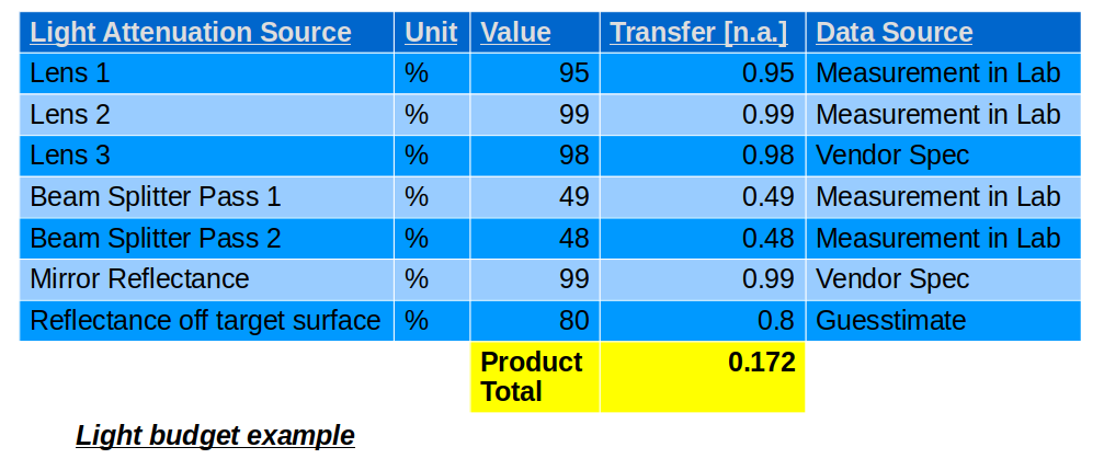
Let’s start with a simple budget example: a light budget. In an optical system, a light budget is the amount of light reaching back to our sensors in [%] from the initial light that originated from the system’s light source. For example, if we have a laser scanning system with a double pass beam splitter (outgoing beam, incoming beam), 3 lenses and a scanning mirror, our light budget will look something like this:
In the budget above the light that will eventually reach the sensor will be 17.2% of the light source, i.e. if we transmitted 1W from the light source we will get in the sensor 172mW. BTW, in this particular system we will have to have another light budget since we have a beam splitter in the middle and that means that there is another light path that has to be taken care of here.
This budget is relatively simple because: (a). most of the rows are with high confidence and (b). most of the optical elements in this table give us a very good light throughput. There is however one guesstimate in the table though but this one guesstimate is out of our control since it is the sample or the target which we are about to measure.
Latency Budget Example
The second example we explore is a latency budget. Latency is the time between two events. Let’s take for example a vision system to tell us what kind of animals, if any, there are in the image and budget the image acquisition and processing latency, i.e. the time it takes from the event of starting grabbing the image in the camera till we get the final answer of the image processing.
The budget will look something like this:
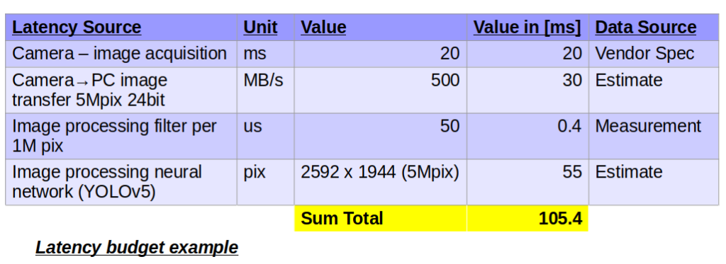
Here we still have a relatively high confidence budget, but note that there are quite a few limitations to keep this budget valid. Since the camera image acquisition is set to 20ms if, for any reason, we have low light we may need to amend this number. The camera→PC image transfer takes into account that we have an 5Mpix camera and that the connection of the camera to the PC is USB3.0 for a 500MB/s data transfer rate. Any change in the camera or camera→PC interface will impact this number and we have to that keep in mind when we start negotiating the different HW we are going to use in our system during design and integration. The same goes for the image processing filter – we measured it on a certain HW but if the HW is replaced we will have to verify this entry and update our budget.
The last row is the most problematic. On the surface it appears to be an ordinary entry, but this estimate, as good as it may be, hides a lot of assumptions behind it. The data for this estimate came from ultralytics YOLOv5, and the reference point was an image 1280 that take 26.2ms to process on a NVIDIA V100, having the estimate taken for about X2 factor for a 2592pix wide image. But wait, a V100 GPU is not exactly a cheap piece of HW (November 2023), and if we are on a tight bill of material (BOM) budget, to switch to CPU will make this entry more than X100 slower, around 6200ms! In cases such as this we should make a note in our budget where the HW dependent entries are and keep them under a close watch.
Optical Signal Error Budget Example
Our third example is a standard error budget for our optical signal. Error budget includes every temporal deviation of a certain attribute that is not systematic, i.e. that cannot be calibrated by the system or by servicing the machine. Anything can contribute to noises and errors: temperature deviation, humidity, electronics, optical effects light interference and speckles, mechanical vibrations, misalignment, anything. In an optical system identical to that in the first example above, the budget, translated into mW of error if the signal is 1W, will look something like this:
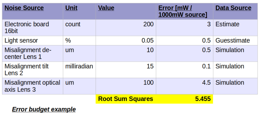
When it comes to error budgets, I always like to use a chart to see exactly which parameters are the budget’s main contributors.
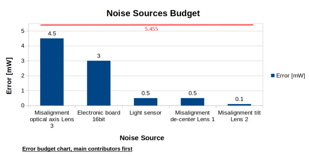
We can clearly see that we have two major error sources, two minor error sources and one negligible error source. We can also see that in the error budgets, the overall error will usually will be the in same order of the main contributors.
You may have noticed that in none of the above examples did I mention whether the budget was good or bad. Good or bad is a matter of requirements. The budget is the technical source to where our design problems are and how close we are technically to the limits. In our third example, if the quantization levels of our optical signal were in the order of 20mW, a ~5.5mW error may be tolerated, but if they were in the order of 10mW we would be forced somehow to reduce the error levels.
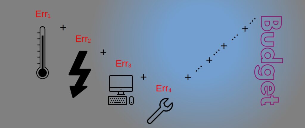
Just remember, even after a very careful calculation of your budget whatever it is, you must leave enough room for additional errors in the budget because of 4 reasons:
- Your Guesstimates – as mentioned earlier, due to limited to no information regarding some of the budget rows we had to guesstimate. These guesstimates endanger the accuracy of the whole budget.
- Unknowns – in complex systems we try to take everything into account, but it is difficult to know it all. We have to leave some room for the things that we did not know that existed in the development.
- Integration changes – during integration things change. We discover parts that do not fit, manufacturing of elements change due to vendors’ capabilities. All these may introduce changes and updates to the different budgets.
- Errors – we are all human (in the meanwhile at least), and only those that do not do, do not make errors. Leave some extra room for human errors.
Obviously the end result of that list may be a better budget eventually, but let’s face it, these are very rare cases and we have to be prepared for the worst case scenario as well as the best case scenario.
I covered a very important system engineering method in this post. The technical budgeting process that is held in the beginning of the project and the budget outcome are the pillars of the design process. Every design input and output have to withstand the relevant budget. The budgeting process is not a one-time event; in every step of the development process, we re-assess the accuracy of our budgets and update it. The calculated budget may even come in handy after we start manufacturing, for troubleshooting manufacturing problems and issues raised by the clients. A well-defined budget may be the difference between a clear and smooth development process and a long and messy one.